Topic outline
-
This course deals with the spreadsheet program, Microsoft Excel. It will take you through the basic features and some of the more advanced uses.
Use of Microsoft Excel
- Working with Cells
- Formatting (including cell types)
- Conditional Formatting
- Basic Formulae
- Print Preview
- Find & Replace
- Sorting
Other Training courses can be found in the Training Category - Working with Cells
-
Working with Cells
Cells work in a very different way from normal text. If you've never worked with them before it can be quite confusing to begin with. This section will act as an introduction to cells and how to work with them.
Navigating
Navigating in excel is broadly similar to other programs. However because of the nature of working with cells (the small boxes that hold information) it can often be easier to use the arrow keys on your keyboard.
All cells are also referenced by their position. They can be found by combining the column and row details. It is always displayed in the top left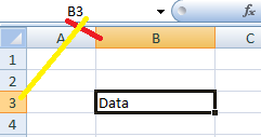
Highlighting
To highlight a particular cell simply click on it. This highlights it with a black box like this:
To highlight a group of cells, click and drag from the first cell to the last without releasing the mouse. Once you've covered them all you can release the mouse. This highlights them as below:
Resizing
To resize a cell you can drag the borders at the top of the cell. In the width example below you need to click and drag on the cell edge, highlighted by the arrow. You can drag it out, and the box appears above to show you how wide the cell is.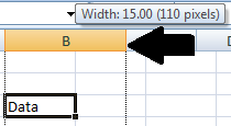
You can equally do this for the height of the cell in the same way.
Double clicking on the border (by the arrow) will automatically resize the cell to fit the contents.
Copying and pasting
To Copy, highlight the cell(s) you wish to copy. Then either press the "Copy" button (below) or press CTRL + C. This will place the cells on the clipboard ready for pasting.
Select the area where you want to paste the data. Then either press the "Paste" button (below) or press CTRL + V.
Filling down/across
To fill down, or across you can click on the small solid square on the highlighted cell, and drag it in either direction. This will copy the data across the selected cells.
A highlighted cell. Note the small black square in the bottom right.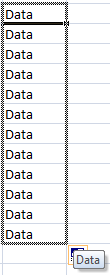
Dragging it downwards copies the cell contents down the entire selection.
-
Formatting
Excel shares a toolbar with a lot of the other office programs, this should make it easy to get used to the formatting in this program.
The font section includes the normal formatting for any document. Changing the font and size just uses the normal drop down menus. Underneath you can make the text bold, italic or underlined. The next box along is different this lets you give borders, click the arrow next to the box to open up the menu giving you a selection or border styles and types.
The alignment section lets you orientate to the left, centre and right as normal. The boxes above this are different for excel, aligning in a cell to top middle or bottom. This is useful if you have large cells. Next to this you can re-orient your texts.
The "Wrap Text" & "Merge and Center" buttons are unique to exchange. Wrap text stops your text from either being hidden or flowing over other cells. It resizes the cells so that all the text can be seen. An example can be seen below.
The Merge text button groups several cells together and links them. This can be very useful for headings and titles. The non merged text is flowing over, and will be hidden if you type into one of the other boxes, the merged text puts those cells together. An example can be seen below.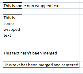
The Number section control the special formatting in excel. The buttons on the left can make the cell a "currency cell" (with the arrow picking the currency) make it a percentage, or insert commas for 1,000 and above. You can also increase and decrease the number of decimal points that display in a cell.
The drop down box at the top (normally general) can let you set a variety of options, examples of them are below. It is worth noting that you need to use "Text" if you want leading 0s, for instance in a phone number. Accounting is also unusual, depending on what you input, it either renders it as currency or a date, but without needing to manually change the type of cell.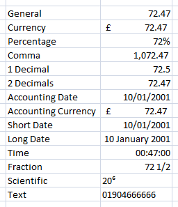
-
Conditional Formatting
Conditional formatting is where the cell can be automatically changed depending on the contents. At the very least you can change the colour to denote things like grades, equally with a bit of work you can get the system to change to visible symbols which can be even more useful.
The below example is a colour scale, it goes from Green to red, with incremental shades for the different scores. As you can see it is very useful to identify marks in a group.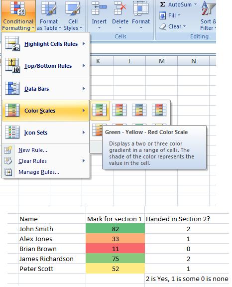
For section 2 we've used a simple system, 2 is Yes, 1 is some, 0 is none of the work handed in. As you can see in the first example some have 2 some 1 and one has 0. We've used an icon set to represent this.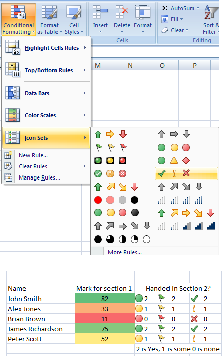
The above example shows 3 different icon sets used commonly, which can give you some ideas. Also if you make the cell small enough, it will display the icon and not the number, looking more streamlined.
-
Basic Formulae
Often when dealing with large amounts of data in excel it can be easier to use formulae to solve problems and perform calculations. This can speed up working, and can even update automatically when the raw data changes.
SUM
SUM is the most basic function in excel. It can be used for totalling sets of figures into the final cell. This can be done in two ways.
You can select specific cells, using the below syntax (specifically , separation). This picks out which ever cells you name, and then totals them.
=SUM(B5,B9,B2)
This selects those cells and adds them.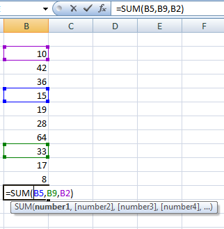
The second way of performing a "SUM" is to total all numbers in a given range. You use the colon (:) to separate the first and last member of the group, excel will then SUM all of the group.
=SUM(B2:B11)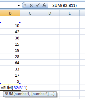
AVERAGE
The AVERAGE function uses similar syntax to the SUM function. You use the same : to contain the cells you wish to average. The average used is the mean of the results.
=AVERAGE(B2:B11)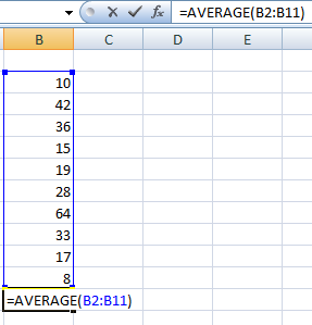
IF
The IF function is a conditional, it lets you test the cells content against a given condition, then returns a true or a false result.
=IF(B2=10,TRUE,FALSE)
=IF(B2>11,YES,NO)
The first section is the condition, this can be any logical condition that returns a true or false. The second section is what is returned if the result is True, and the third section is returned if the result is False. The sections are separated by the commas.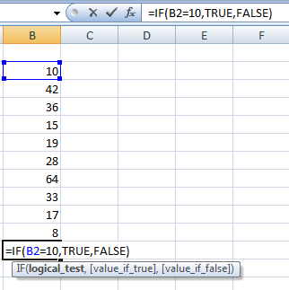
COUNT
The COUNT function in excel returns the total number of cells with numerical data in. This can be useful if you wanted to know how many students work had been marked, simply issue a count function on the line of results and excel will tell you how many are filled. It uses the same syntax as AVERAGE & SUM.
=COUNT(B2:B11)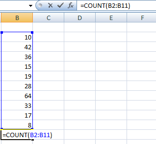
MAX
The MAX function returns the highest value in a given range. The syntax is similar to AVERAGE & SUM, but returns the highest numerical value. It ignores text or logical arguments.
=MAX(B2:B11)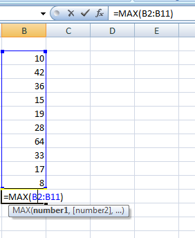
AND (logical)
The logical AND function returns TRUE if all the fields are TRUE (TRUE or 1) and FALSE otherwise. The syntax follows the common SUM syntax.
=AND(B2:B3)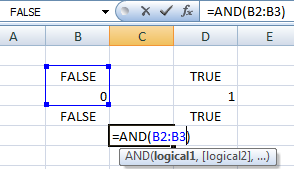
OR (logical)
The Logical OR function returns TRUE if any or all of the fields are TRUE (TRUE or 1) and FALSE if they are all FALSE. The syntax follows the common SUM syntax.
=OR(B2:B3)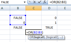
Function Menu
The function menu is your repository for all the possible functions in excel. You can search them, or look at the categories in a drop down list. Each one also has an explanation of the syntax beneath. You can access the menu by pressing the fx button highlighted below.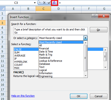
-
Using Print Preview in Excel
Print preview can be used to check how the spreadsheet will print out. This is common to most office suites, but can be particularly useful in excel. Clicking on file then print, or CTRL and F2 will open the print window. On the right hand side of this is a preview of what your printout will look like.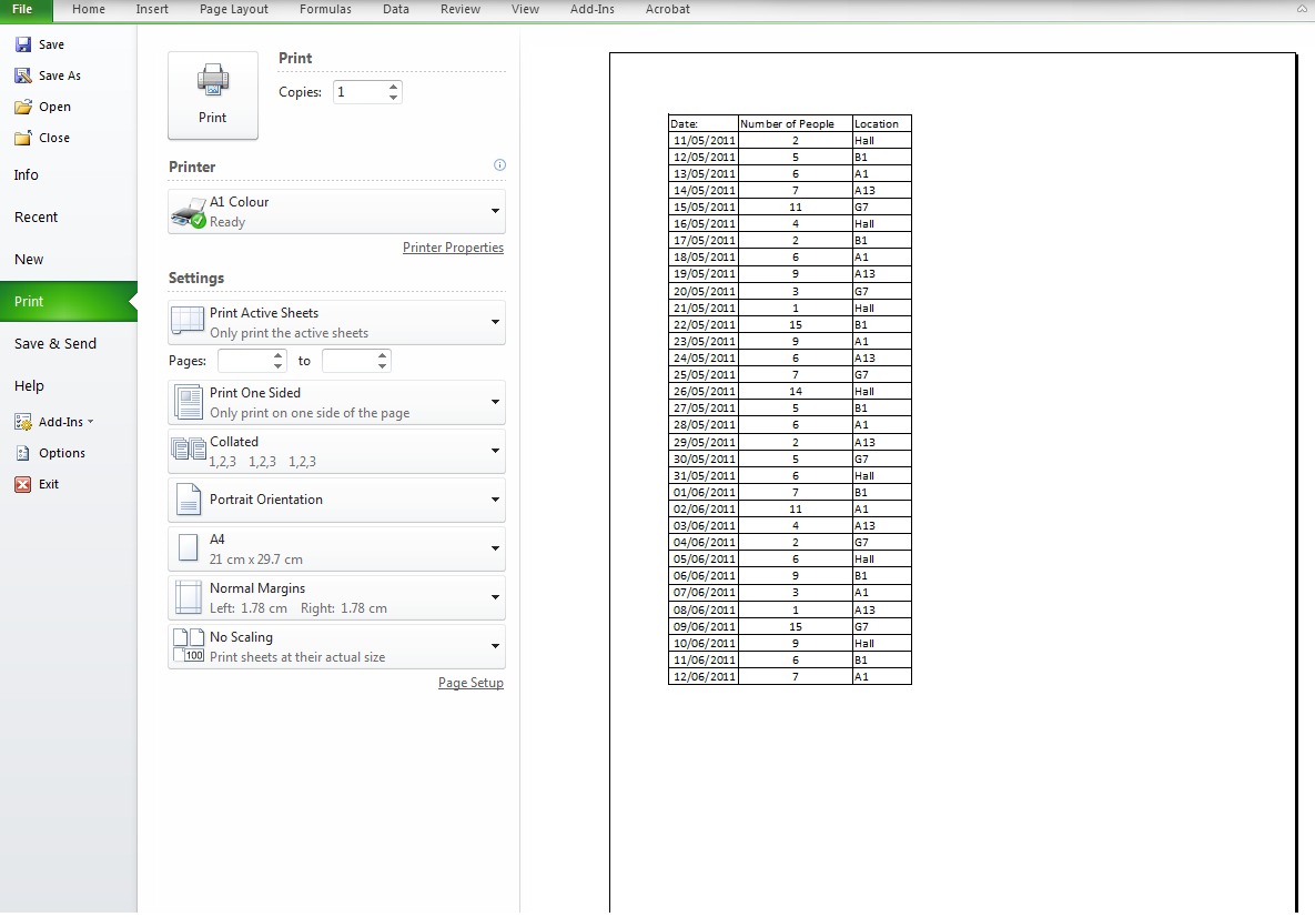
This will let you see how the spreadsheet will print out. Once you close this (by using the x in the top right) you are returned to the spreadsheet.
Once you've used the print preview a change will have been made to the spreadsheet, the area that will be printed will be highlighted by dotted lines as below. This can be useful as you edit to see what will be printed.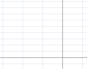
-
Find and Replace
Basic Finding
The basic find menu can be activated by pressing CTRL and F. This brings up the below window. You can type in your search term, pressing enter will make excel find the next instance of this term, and you can press next to cycle through them.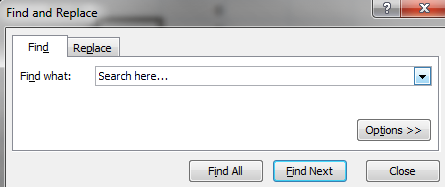
Find & Replace
The full find and replace menu has lots of options. You can change the formatting, to search by formatting (e.g. all bold text) or replace the text with formatted text. You can also match the case, or search for all or part of the contents.
The replace box is what will be filled in, you can format this with the formatting box.
With the bottom buttons you can "Find All" instances, "Find Next" to locate the next one. You can "Replace" the currently highlighted one, or "Replace All" to automatically go through all of the sheet making the changes.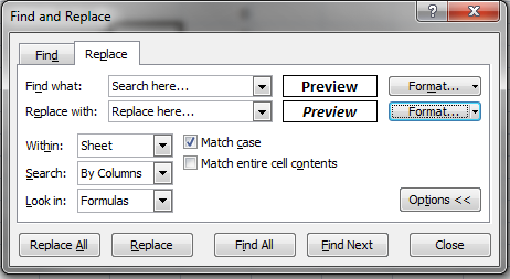
-
Sorting
Basic sorting
The basic sort buttons sorts the selected data from A to Z or Z to A. This can be useful for quickly sorting lists of data like surnames.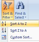
Full sort menu
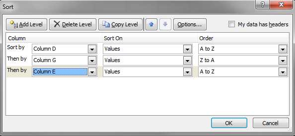
The full sort menu is more exhaustive, this can help sort out different types of data. For students names it can sort by surname then forename.
Clicking "Custom sort" opens up the sort window. This will sort by a column, you can change which one and whether its A to Z or Z to A. You can Add a level using the top left button, and then sort by an additional column.